{
"cells": [
{
"cell_type": "markdown",
"metadata": {},
"source": [
"# Lecture 9 (guest) - Data Visualization with Seaborn"
]
},
{
"cell_type": "markdown",
"metadata": {},
"source": [
"## Seaborn\n",
"\n",
"**`Seaborn`** is a data visualization library built on the top of `matplotlib`. It was created by [Micheal Waskon at the Center for Neural Science, New York University](https://joss.theoj.org/papers/10.21105/joss.03021).\n",
"\n",
"**`Seaborn`** has all the attributes of the `matplotlib` library (it is a child class), making it considerably easy to plot data using Python.\n",
"\n",
"We will learn some of these plots in this class and a few customizations. More about `Seaborn` can be found in [here](https://seaborn.pydata.org).\n",
"\n",
"Below you can find a list of functions that we can use to plot data on `Seaborn`.\n",
"\n",
"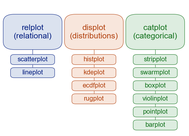"
]
},
{
"cell_type": "code",
"execution_count": 1,
"metadata": {},
"outputs": [],
"source": [
"# Importing libraries\n",
"import pandas as pd\n",
"import numpy as np\n",
"import matplotlib.pyplot as plt\n",
"import seaborn as sns # This is how you import seaborn\n",
"\n",
"# Datasets\n",
"\n",
"## Political and Economic Risk Dataset\n",
"# Info on investment risks in 62 countries in 1992\n",
"# courts : 0 = not independent; 1 = independent\n",
"# barb2 : Informal Markets Benefits\n",
"# prsexp2 : 0 = very high expropriation risk; 5 = very low\n",
"# prscorr2: 0 = very high bribing risk; 5 = very low\n",
"# gdpw2 : Log of GDP per capita\n",
"perisk = pd.read_csv('https://raw.githubusercontent.com/umbertomig/seabornClass/main/data/perisk.csv')\n",
"perisk = perisk.set_index('country')\n",
"\n",
"## Tips Dataset\n",
"# Info about tips in a given pub\n",
"# totbill : Total Bill\n",
"# tip : Tip\n",
"# sex : F = female; M = male\n",
"# smoker : Yes or No\n",
"# day : Weekday\n",
"# time : Time of the day\n",
"# size : Number of people\n",
"tips = pd.read_csv('https://raw.githubusercontent.com/umbertomig/seabornClass/main/data/tips.csv')\n",
"tips = tips.set_index('obs')"
]
},
{
"cell_type": "markdown",
"metadata": {},
"source": [
"And here is what we have in these datasets:"
]
},
{
"cell_type": "code",
"execution_count": 2,
"metadata": {},
"outputs": [
{
"data": {
"text/html": [
"\n",
"\n",
"
\n",
" \n",
" \n",
" | \n",
" courts | \n",
" barb2 | \n",
" prsexp2 | \n",
" prscorr2 | \n",
" gdpw2 | \n",
"
\n",
" \n",
" | country | \n",
" | \n",
" | \n",
" | \n",
" | \n",
" | \n",
"
\n",
" \n",
" \n",
" \n",
" | Argentina | \n",
" 0 | \n",
" -0.720775 | \n",
" 1 | \n",
" 3 | \n",
" 9.690170 | \n",
"
\n",
" \n",
" | Australia | \n",
" 1 | \n",
" -6.907755 | \n",
" 5 | \n",
" 4 | \n",
" 10.304840 | \n",
"
\n",
" \n",
" | Austria | \n",
" 1 | \n",
" -4.910337 | \n",
" 5 | \n",
" 4 | \n",
" 10.100940 | \n",
"
\n",
" \n",
" | Bangladesh | \n",
" 0 | \n",
" 0.775975 | \n",
" 1 | \n",
" 0 | \n",
" 8.379768 | \n",
"
\n",
" \n",
" | Belgium | \n",
" 1 | \n",
" -4.617344 | \n",
" 5 | \n",
" 4 | \n",
" 10.250120 | \n",
"
\n",
" \n",
"
\n",
"
\n",
"\n",
"
\n",
" \n",
" \n",
" | \n",
" totbill | \n",
" tip | \n",
" sex | \n",
" smoker | \n",
" day | \n",
" time | \n",
" size | \n",
"
\n",
" \n",
" | obs | \n",
" | \n",
" | \n",
" | \n",
" | \n",
" | \n",
" | \n",
" | \n",
"
\n",
" \n",
" \n",
" \n",
" | 1 | \n",
" 16.99 | \n",
" 1.01 | \n",
" F | \n",
" No | \n",
" Sun | \n",
" Night | \n",
" 2 | \n",
"
\n",
" \n",
" | 2 | \n",
" 10.34 | \n",
" 1.66 | \n",
" M | \n",
" No | \n",
" Sun | \n",
" Night | \n",
" 3 | \n",
"
\n",
" \n",
" | 3 | \n",
" 21.01 | \n",
" 3.50 | \n",
" M | \n",
" No | \n",
" Sun | \n",
" Night | \n",
" 3 | \n",
"
\n",
" \n",
" | 4 | \n",
" 23.68 | \n",
" 3.31 | \n",
" M | \n",
" No | \n",
" Sun | \n",
" Night | \n",
" 2 | \n",
"
\n",
" \n",
" | 5 | \n",
" 24.59 | \n",
" 3.61 | \n",
" F | \n",
" No | \n",
" Sun | \n",
" Night | \n",
" 4 | \n",
"
\n",
" \n",
"
\n",
"
\n",
"\n",
"
\n",
" \n",
" \n",
" | \n",
" polInf | \n",
" collegeDegree | \n",
" female | \n",
" age | \n",
" homeOwn | \n",
" govt | \n",
" length | \n",
" id | \n",
"
\n",
" \n",
" \n",
" \n",
" | 0 | \n",
" Fairly High | \n",
" Yes | \n",
" No | \n",
" 49.0 | \n",
" Yes | \n",
" No | \n",
" 58.400002 | \n",
" 1 | \n",
"
\n",
" \n",
" | 1 | \n",
" Average | \n",
" No | \n",
" Yes | \n",
" 35.0 | \n",
" Yes | \n",
" No | \n",
" 46.150002 | \n",
" 2 | \n",
"
\n",
" \n",
" | 2 | \n",
" Very High | \n",
" No | \n",
" Yes | \n",
" 57.0 | \n",
" Yes | \n",
" No | \n",
" 89.519997 | \n",
" 3 | \n",
"
\n",
" \n",
" | 3 | \n",
" Average | \n",
" No | \n",
" No | \n",
" 63.0 | \n",
" Yes | \n",
" No | \n",
" 92.629997 | \n",
" 4 | \n",
"
\n",
" \n",
" | 4 | \n",
" Fairly High | \n",
" Yes | \n",
" Yes | \n",
" 40.0 | \n",
" Yes | \n",
" No | \n",
" 58.849998 | \n",
" 4 | \n",
"
\n",
" \n",
"
\n",
"
\n",
"\n",
"
\n",
" \n",
" \n",
" | \n",
" Murder | \n",
" Assault | \n",
" UrbanPop | \n",
" Rape | \n",
"
\n",
" \n",
" \n",
" \n",
" | 0 | \n",
" 13.2 | \n",
" 236 | \n",
" 58 | \n",
" 21.2 | \n",
"
\n",
" \n",
" | 1 | \n",
" 10.0 | \n",
" 263 | \n",
" 48 | \n",
" 44.5 | \n",
"
\n",
" \n",
" | 2 | \n",
" 8.1 | \n",
" 294 | \n",
" 80 | \n",
" 31.0 | \n",
"
\n",
" \n",
" | 3 | \n",
" 8.8 | \n",
" 190 | \n",
" 50 | \n",
" 19.5 | \n",
"
\n",
" \n",
" | 4 | \n",
" 9.0 | \n",
" 276 | \n",
" 91 | \n",
" 40.6 | \n",
"
\n",
" \n",
"
\n",
"